Information collection engines such as the one that helps Amazon customers find products in the Amazon store are often dependent on bipartite graphs that map queries for products. The graphs are typically based on customer behavior: If enough customers carry out the same query, click the link to a product or buy that product, the graph will contain an edge between query and product. A graph of neural network (GNN) can then consume the graph and predict edges corresponding to new queries.
This approach has two disadvantages. One is that most products in the Amazon store belong to the long tail of items that are rarely searched for, which means they do not have enough associated data to make GNN training reliable. Conversely, when handling long-tail queries, a GNN tends to match them to popular but probably non-related products simply because they generally have a high click and purchase speed. This phenomenon is known as Removative mixture.
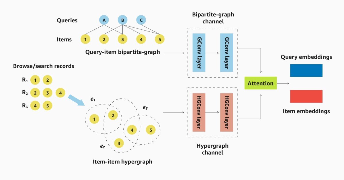
In a paper we presented at the ACM conference on the Web Search and Data Mining (WSDM), we solve both of these problems by increasing Bipartite request product graph with information about what products customers tend to look at during the same online shopping sessions. The idea is that knowing what types of products are related to each other can help GNN generalize from high frequency to low -frequency queries.
To capture the information about product conditions we use a Hypergrapha generalization of the graph structure; Where an edge in an ordinary graph connects exactly two nodes, an edge in a hypergraf can connect several nodes. Other information collection methods have used productivity to improve performance, but modeling of productability with the hypergrafen allows us to use GNNs for prediction so that we can utilize the added structure available in data graphic representations.
In Tests, we compared our approach to someone who only uses GNNs on a bipartite graph and found that the addition of the hypergrafen improved the average mutual rank of the results that assigns a higher score, the closer the correct answer is on the top of a ranked list, with almost 25% and recall score measuring the percentage of the correct answers that are repaid, with more than 48%.
Two-channel architecture
GNNs produce vector representations or embedders of individual graphs that capture information about their neighbors. The process is iterative: The first embedding only captures information about the object associated with the node – in our case product descriptions or query semantics. The second embedding combines the first embedding with them from the nod’s closest neighbors; The third embedding extends the Node’s neighborhood with a jump; And so on. Most applications use one or two-hop deposits.
The embedding of a hypergraf changes this procedure slightly. The first iteration, as in standard cases, embedes each of the product nodes individually. The other iteration creates a embedding for the whole hyperge. The third iteration then produces an embedding for each nodule that factors in both its own content of content and embedders of all the hyperedges it touches.
The architecture of our model has two channels, one for the inquiry topic bipartite graph and one for the product topic hypergraf. Each is transferred to its own gnn (a graphomic convolution network), giving a embedding for each knot.
During training, an attention mechanism learns how much weight he has to give the embedding produced by each channel. For example, a regular inquiry with a few popular affiliated products may be well represented by standard GNN gnawing of the bipartite graph. A rarely purchased item, on the other hand, associated with a few different queries, can benefit from greater weighting of the hypergraf injury.
To maximize the quality of our model’s predictions, we also experimented with two different unattended prior methods. One is a contrasting learning method where GNN is fed with pairs of training examples. Some are positive couples whose embedders should be as similar as possible and others are negative couples whose embedders should be as different as possible.
After existing practice, we produce positive couples by randomly erasing edges or nodes on a source graph so that the resulting graphs are the same but not identical. Negative couples pair the source graph with another, random graph. We extend this procedure to the hypergrafen and ensure consistency between the two channel training data; E.g. Deleted a knot that has been deleted from one channel’s input, also from the other channel.
We also experiment with droping, a procedure where in successive training poker slightly different versions of the same graph, with a few edges, randomly fell. This prevents over -consuming and over -consumption as it encourages GNN to learn more abstract representations of its input.
Pretraining dramatically improves the quality of both our two-channel model and baseline gnn. But it also increases the discrepancy between the two. That is, our approach of itself sometimes only provides a modest improvement over the baseline model. But our approach to prior, the baseline model exceeds prior to a larger margin.