The prices of products in the Amazon store reflect a number of factors, such as Dequest, seasonal provision and general financial trends. Price policies typically involve formula that take into account such factors; Recent pricing policies are unsaltable on machine learning models.
With Amazon Pricing Labs we can lead a number of online A/B experiment to evaluate new pricing policies. Because we practice pricing of non -discrimination – all visitors to the Amazon store at the same time see the same prices for all products – we have to use experimental treat For product prices over time, rather than testing different price points simultaneously on different customers. This complicates the experimental design.
In a paper we published in Journal of Business Economics In March and presented at the American Economics Association’s annual conference in January (AEA), we described some of the experiences we can lead to emissions, improve precision and control for demand trends and various treatment groups when assessing new pricing policies.
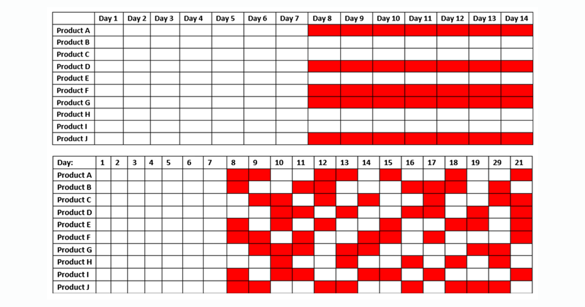
The simplest type of experiment we can perform is a Time -tied Experiment where we apply a treat on a product in a particular class while leaving other product in the class untreated, as checks.
A potential noise source in this type of experience is that an external event – says, a temporal discount on the same product in another store – can affect treatment effects. If we can define these types of events in advance we can lead Triggered interventionsWhere we have time to start with our treatment and control periods for the events. This can result in staggered start time for experience is different.
If the demand curves for the products are the same enough and the different in the results between the treatment group and the control group is dramatical enough, time -tied and triggered experiment may be sufficient. However, for a more accurate evaluation of a pricing policy, it may be necessary to run treatment and control experience on the same product as would be the case with typical A/B test. It requires it Switchback Experiment.
The most straight -prompt Switchback -Experiment is random Experiment where each product is randomly assigned to the EITH control group or the treatment group every day. Our analyzes indicate that random days can reduce the standard error in our experience results – that is, the extent to which the statistics of our observations are different from true statistics of the intervention – by 60%.
However, one of the disadvantages of any Switchback experiment is the risk of TransferWhere the effects of a treat are transferred from the treatment phase of the experience to the control phase. For example, if randoms are treated a product’s sales, algorithms recommendation recommend this product more often. It could artificially increase the product’s sales even during control periods.

We can combat the transfer of institutes blackout periods during transitions to treatment and control phases. In one Crossover experimentFor example, we may be able to do apps a treat for a product in a group, the others as controls, but throw away the first week’s data for both groups. Then, after collecting enough data – e.g. Two weeks value – we remove the processing from the form’s treatment group and apply them on the form. Once again, we throw out the first week’s data to let the transfer effect die down.
Crossover experiment can reduce the standard error in our performance measurements by 40% to 50%. It is not as good as random days, but transfer effects are mitigated.
Heterogeneous panel treatment effect
The Amazon Price Laboratories also offer two more sophisticated funds to evaluate pricing policies. The first of these is the heterogeneous panel treatment effect or HPTE.
HPTE is a four-step process:
- Estimates product level first difference from detailed data.
- Filter Outliers.
- Other differences are estimated from grouped products using causal forest.
- Bootstrap -data to estimate noise.
Estimates product level first difference from detailed data. In a standard Different-in-Dift (DID) analysis, the first different different is between the results of a single product before and after the experience begins.

Instead of simply drawing the results before treatment from the results after treatment, however, we analyze historical tendencies to predict what ALD has had if products were left untreated during the treatment period. We then draw the perpetrated from the observed results.
Filter Outliers. In the price experiment, there are often Unobnate factors that can cause extreme swings in our results. We define a Cutoff point for Outliers as a percentage (quantity) of the performance distribution that is inversely proportional to the number of products in the data. This approach has been used in the past, but we validated it in simulations.
Other differences are estimated from grouped products using causal forest. In DID analysis, the second difference is the difference between the first differences of treatment and control groups. Becuse We consider groups of heterogeneous products, we calculate the other difference only for product that has strong enough affinities with each other to make the comparison informative. Then we average the other difference across products.
In order to calculate affinity results, we used to variation on decision trees called Causal guys. A typical decision tree is a connected acyclic graph – a tree – each whose nodes represent a question. In our case, these questions consider product characteristics – say, “Does the interchangeable batteries require?”, Or “Is its width greater than three inches?”. The answer to the question decides which branch of the tree to follow.
A causal forest consists of many such trees. The questions are taught by the data and they define the axes that the data shows the largest variance. Therefore, the data used to train the requirements is no labeling.
After training in causal forest, we use it to evaluate the product in our experience. Products from treatment and control groups that end up by the Sans -Terminal Nudse or Leaf are considered by a tree as similar enough for their other difference to be calculated.
Bootstrap -data to estimate noise. To calculate the default error, we randomly try products from our data set and calculate their average processing power, then return them to the data set and try randomly again. More resampling allows us to calculate the variance in our outcome measurements.
Spillover effect
At the Amazon price laboratories, we have also investigated ways of measuring the overplay effect that arises when the treatment of a product causes a change in demand for another, similar product. This can throw off our measurements of the treatment effect.
For example, if a new pricing of the policy increases the demand for, for example, a particular kitchen meat, more customers will see this Flesh’s product page. However, some fraction of these customers may buy another chair listed in the page’s section “Discover similar items”.
If the other chair is in the control group, its sales can be artificially significant in the treatment of the first meat, leading to an underestimation of the treatment effect. If the other meat is in the treatment group, the inflation of its sales can lead to a overEstimate of the treatment effect.
To correct for the overplay effect, we need to measure it. The first step of this process is to build a graph of products with correlated demand.
We begin with a list of products related to each other in accordance with criteria, such as their fine-grained classifications in the Amazon store catalog. For each pair of related items, we then look at the one year’s value of data to determine if a change in the price of one employment for another. If these connections are strong enough, we will join the products at an edge in OU-Substituing points.
From the graph, we calculate the likelihood that anyone will give pairs of substitutable products will find themselves in the same experience and what group, treatment or control they are assigned. From these probabilities, we can use reverse probability weight scheme to estimate the effect of waste on observed results.
However, it is not as good to estimate wastewater effect as eliminating it. One way to do this is to be substitutional productable products as a single product class and assign them to treatment or control groups a lot. This reduces the power of our experience, but it gives our business partners confidence that the results are not toned by waste.
To determine which products to include in each of our product classes, we use a cluster algorithm that searches the replacement product graph for regions with close interconnection and separates these regions connections to the rest of the graph. In an iterative process partitions this graph in clusters of closely related products.
In simulations we found that this cluster process can reduce waste bias by 37%.