One of the lessons in the Machine Learning Revolution has been that perhaps resistant, to educate a model of multiple data types or multiple tasks can improve the relative performance of one-facing models. A model trained in multiple languages, for example, can lead to distinctions that are subtle in one language, but pronounced in another, and a model that is trained on, says object segmentation can learn the properties of visual scenes that help it with in -depth perception.
However, the advantages of multitask and multimodal training are relatively unprocessed in the context of diffusion models, which are responsible for some of the most impressively recent results in generative AI. Diffusion models are trained for step -by -step denoise samples for which noise is inserted. The result is that feeding them random noisy input will provide randomized output that is semantically coherent.
In a paper we presented at the international conference on learning representations (ICLR), we describe a general approach to building multimodal, multitask diffusion models. On the input side, we used modality security coders to map data to a shared diffusion space; On the output side, we use several task parcoders to map general representations to specific output.
The paper presents a theoretical analysis of the problem of generalizing diffusion models to the multimodal, multitasking setting, and on the basis of this analysis it suggested several changes to the loss function typically used for dissemination modeling. In the experiment, we tested our approach on four different multimodal or multitask data sets, and everywhere it was able to match or improve the relative performance of single-formless models.
Memorial modality
In the standard diffusion modeling scenario, the model codes enter the codes of a Represh room; Within this space, a forward -looking process adds iterative noise to the input representation and a reverse process removes it iteratively.

The loss function includes two expressions that measure the distance between the probability distribution of the forward process and the learned probability distribution of the reverse process. An expression compares Marginal distribution For the two processes in the front direction: That is, it compares the probabilities that any given noisy representation will occur during the future process. The second expression compares the posterior representations of the inverted process – that is, the likelihood of a give representation on time T-1 Prior to the representation at the time T.. We change these expressions so that the distributions are contingent on the modality of the data – that is, the distributions may vary for data from different modalities.
Both of these loss conditions operate in the representative space: they consider the likelihood of a particular representation considering another representation. But we also have an expression in the loss function that looks at the likelihood that an input of a given modality led to a particular representation. This helps to ensure that the reverse process correctly restores the modality of the data.
Multimodal means
To merge the multimodal information used to train the model, we are considering the transitional distribution in the front direction, which determines how much noise to add to a Give Date presentation. To calculate the average of this distribution, we define a weighted average of the multimodal input codes where the weights are based on input modality.
Based on the transition probability of the forward process, we can now calculate the marginal distribution of noisy representations and the rear distributions of the reverse process (similar to lower lengths L.0 and L.1 In the Tab function):
Assessment
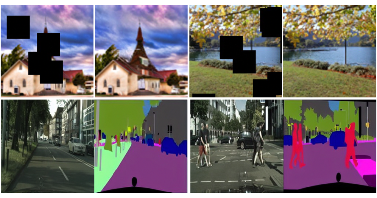
We test for the approval of four tasks, two of which were multitask, and two of which were multimodal. The multitask experiment was both in the vision domain: one involved jointly generating visual data and the associated segmentation masks, and the other was a new multitask testing task, where a diffusion generation model also learned filling in masked regions with input images.

The multimodal experiment involved images and other modalities. In one, the model was trained to jointly generate images and their labels, and in the other the model learned to generate images and their embedders in a representing space – for example, clips embedders.
The image segmentation was and embedded generation tasks were mainly intended for qualitative demonstrations. But the masked prior task and the common generation of images and labels enabled quantitative evaluation.
We evaluated the masked Pretrache model on the task of resuming the masked image regions using learned perceptual image plastic equality (LPIPS) as a metric. LPIPS measures the similarity between two images according to their activations of selected neurons within a picture recognition model. Our approval dramatically exceeds the basic lines that were only trained in the reconstruction task, not (at the same time) on the diffusion task. In some boxes, our model failure rate was almost an order of magnitude lower than the baseline models.
On the task of generating images and labels together, our model performance was comparable to that of the best baseline-vision-Langage model with slightly higher precision and slightly lower recall.
For this original experience, we assessed multitask and multimodal performance separately, and each experience involved only two modalities or tasks. But at least prospectively, the power lies in our model in its generalizability, and in nursing work we evaluate on several two modalities or tasks at the time and at the same time multitas and multitask training. We are eager to see the result.