Anomali detection is the identification of data that differs significantly from established norms, which may indicate damage activity. It is a particularly tough challenge in the case of graph -based data, where anomalid detection is not only based on data values, but on topological conditions with the graph. Becuse anomalies tend to be rare, it can be difficult to find enough examples to train a machine learning model on the complexity of anomaly detection in graphs.
In a paper we presented last week at the International Conference on Web Search and Data Mining (WSDM), we describe a new method of synthesis of training data for graph -based anomalidetectors. Our method combines a variation graph autoCoder that learns a probability distribution that can be used to generate random samples, with diffusion modeling that learns to convert random noise into understandable output.
In Tests, we compared anomalidetectors trained with synthetic data generate through our method of detectors that were trained Facting Five Previous Announcements for Data Increase. We compared the models on five data sets using three different measurements for a total of 15 experiment. In 13 of these experiment, our model came on top; Different models were the best artists on the other two.
Graph -based modeling
Graphs are the natural way of absorbing data movement through networks where the computer networks, communication networks or networks of interactions, as between buyers and sellers on an e-commerce website. Thus, anomaly detection in graphs can help detect server attacks, spam, fraud and other types of abuse.
In recent years, graph analysis, like most fields, has benefited from deep learning. Graf Neural Networks builds graph representations iteratively: First, they integrate the data similar to the graph; Then they produce embedders that combine knot inlets with those with adjacent nodes; Then they produce embedders that combine these high -level embedders; And so on, une something fixed termination point. Ultimately, the model produces embedders that capture information about the entire neighborhoods of the graph. (In our experience, we decided for ovenhop neighborhoods.)
The complexity of graphs – the need to take data both topologically and quantitatively – means that models for analyzing they need extra training data that can be scarce in nature. Therefore, the need for synthetic training data.
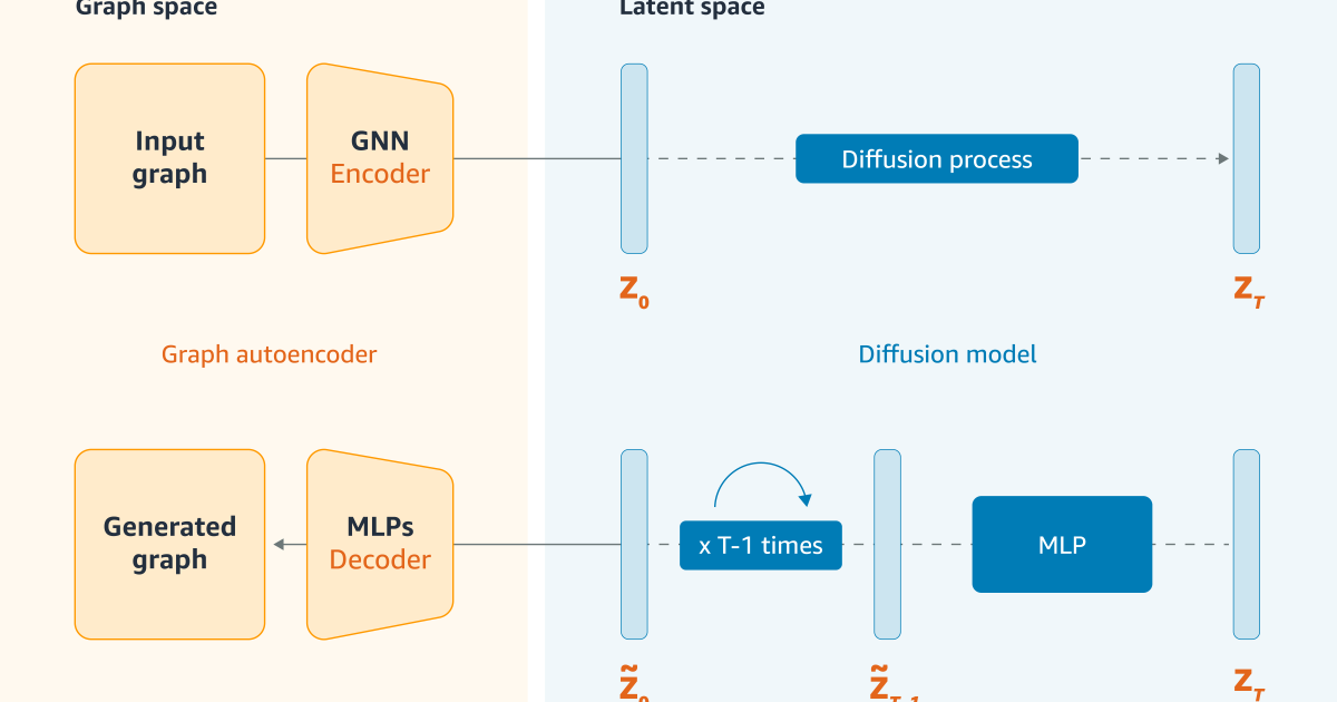
Latent space diffusion
At its core, our data synthesis model is a variation graph autoCoder. “AutoCoder” means it is trained to send out the same data it receives as input. Between the input and output layers, Howwever, is a bottleneck layer that forces the network to learn a compressed representation of input.
“Variement” means that the model’s training goals that encourage it not only to reproduce input but also to the compressed representations whose distribution adheres to some anti -tea pre -determined form, such as a Gaussian distribution. This means that it is likely to result in realistic data, to operate the data synthesis phase and result in realistic looking data.
AutoCoders compressed representations define a representative space, and it is with the space that we use modeling. AutoCoder produces an embedding of the input graph and our model iteratively adds noise to it. To be the performance the same process in reverses that iteratively can denoize the embedding.
This is effective another control to ensure that the synthetic data is similar to real data. If the distribution taught by the autoCoder is not capturing the properties of analysis data, the addition of noise can “blur out” the ski -acidic functions. The Denoising step then fills the blurred features with features more consists of the training data.
Data synthesis
Our approval has a few other warkles designed to improve the quality of the synthesized data. One is that after the diffusion process passes the reconstituted graph that embedes not one but more decores, each specialized to another aspect of the graph.
At least there are two decoders, one for knot functions and one for graph structure. If the graphs in question include time series data, we use a third decode to assign timestamps to nodes.

Another wrinkle is that during training we notice graph nodes such as anomal or normal and then train on both positive and negative examples. This helps the model learn between the two distinctions. But it also means that the model learns a distribution conditioned by class labels, so awake synthesis, we can control it against samples that will result in graphs that contain deviations.
It was fine, it was important that our model could generate heterogeneous graphs – that is, graphs with different node and edge types. In an e-commerce setting, for example, nodes may take buyers, sellers and product pages, while edges can resume purchases, product views, reviews and the like.
As the cod in our autoCoder, we use a heterogeneous graph transformation, A, which have been several modifications to enable it to handle heterogeneous graphs, included separate attention mechanisms for different nodes or edge types.
Overall, these features in our model are able to surpass its predecessors, and in the paper we report an ablation study showing that each of these features that contributes significantly to our model’s success.