At the same time, location and mapping (sludge) are the core technology of autonomous mobile robots. At the same time, it involves building a map of the robot’s environment and finding the robot’s location within this map.
Sludge is calculated intensive and implements it on resource-limited robots-as consumers’ household robots-generally technical requirements to make calculations more dragging.
Such a technique is the use of low -precision -flowing arithmetic or reducing the number of bits used to take numbers with decimal points. The technique is popular in deep learning, where halving the number of bits (from standard 32 to 16) can double calculation efficiency with low effect on accuracy.
But applying low precision arithmetic to sludge is more complicated. Where dy bladder-based classification models are discreet values, sludge involves solving a non-linear optimization problem with continuous valued functions that require higher accuracy.
At Amazon, we have tackled this problem by designing a new Solver-Prison Solver that combines 64-bit (FP64), 32-bit (FP32) and 16-bit (FP16) trials for non-linear optimization problems in the slam algorithm. This innovation paves the way for faster and greener navigation on devices.
General framework
A sludge -algorithm has two key components: Visual kilomenia thread and loop closure. Visual kiloma harvesting provides real -time estimates of the robot’s pose or its orientation and rent on the map based on the latest observations. When the robot acknowledges that it has arrived at a place that it previously visits, the Closes the loop By Globillaly correcting his card and its rent estimate.
Both Visual Odumetry and Loop closure involve the solution of non -linear optimization problems -bundle adjustment (BA) and constitute graph optimization (PGO), respective. To solve them effectively, sludge systems typically use approximate methods that are reworked them as sequences of linearized optimization problems. If the goal is to find the position estimate XThen each linear problem minimizes the linearized malfunction which is the sum of the current malfunction and its first order correction. The first order correction is the product of Jacobian, which is the matrix for the first derivative of the function and the update to the estimation. The linear problems are typically solved through factorization using either cholsky or QR methods. The solution of each linearized optimization problem is the update to the current position.
The general procedure is to start with the current approximation of XCalculate the malfunction and jacobian, solve a linear optimization problem and update X Accordingly, the process repeats until the stop criteria are met. At each iteration, the value of the malfunction is known as remainingSince it is the remaining mistake that is left from the previous iteration.
The most expensive calculations in the non -linear optimizations for both BA and PGO are the calculation of Jacobian (about 15% of the optimization time) and the solution of the linear problem (about 60%). Just solving either problem at semi -precision (FP16) from beginning to finish will result in lower accuracy and sometimes numeric instabilities.
To mitigate these difficulties, we rain and scale the matrixes to avoid overflow and rank deficiency. The rank error occurs when columns in Jacobian are linearly depends. Through carefully experiment, we further identified the calculations to be performed at precision higher than FP16 and suggested mixing non-linear optimization of mixed prote optimization.
We found that to match the accuracy of the solution in pure double precision, the following two components must be calculated in precision higher than FP16:
- The remaining must be evaluated in single or high precision;
- The update of XWhich is a six-degree position angle update, must be in double precision.
Although this general optimization framework is used for both BA and PGO, the details vary across the two applications due to the different structures and properties of the matrixes in the linear problems. We thus offer two mixed precision solution strategies for the relevant linear systems.
Visual kiloma hair
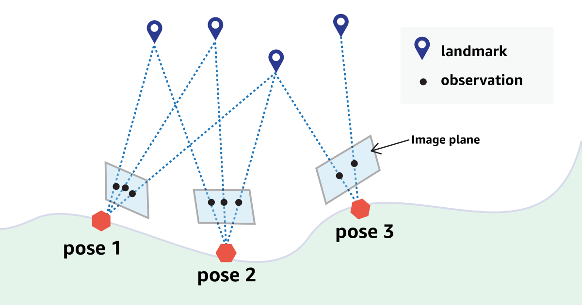
For visual kiloma harvesting, people traditionally use filter -based methods that may suffer from great linearization errors. Non-linear optimization-based methods have become more popular in recent years. These methods estimate the position and orientation of the robot by minimizing a malfunction that is different between re -proofing of landmarks and their observation in the picture frame. This procedure is called bundle adjustment because we add a bundle of light rays that match the projection with the observation.
BA-based visual kilomethometi works over a shooting game containing a fixed number of (key) frames. We carry, in a new key frame comes at 10Hz. The challenge is to solve the BA problem within a given time budget. A popular way of doing this is to solve the normal equation that corresponds to the linearized optimization problem; This involves the approximation of the Hessian matrix or the matrix of second -order derivatives of the remaining.
The BA problem involves two sets of unknown state variables: One indicates the robot’s pose and the other indicates landmark rental. One way to reduce the calculation burden of the BA problem is to marginalize the limitations between camera positions and landmarks and focus first on the camera bags. In the Slam -Society this procedure nown is like Schur Elimination gold Landmark marginalization.
This marginalization step can reduce the size of the linear system to be solved. For a BA problem of 50 frames, the Jacobian matrix is usually of size 5,500 x 1,000, and Hessian is of size 1,000 x 1,000. Disclosure of restrictions reduces the size of the linear system to 300 x 300, small enough to be resolved with direct or iterative solvers. However, this strategy requires both the formulation of the Hessian matrix and a partial elimination step that is expensive for employment in practice.
Our Mixed-Price Linear Solver, which mixes simple and semi-precision, is based on the conjugate gradient normal equation resort (CGNR) method, which is an ethod that is directly used for the linear optimization problem without explicit by Hessian.
As in the general framework, a naive casting of all calculations for semi -precision will result in low accuracy. In our experience, we found that if we calculate matrix vector products in semi-precision and all other operations in single precision, we will keep the total accuracy of the sludge pipeline.
The Matrix Vector Products, which are the most important calculation in CNGR ITEIRATIONS, USLly Center for 83% of computer costs in terms of the number of liquid dot operations. This means that if it is run on the NVIDIA V100 GPUs, the mixed fast-solver could save at least 41% solution time compared to the single precision linear solver.
Loop closure
In the SLAM pipeline, the local postures from Vo Uslely show great operation, especially in the long run. LOOP closure corrects this operation.
For an estimate of mapping the real world without LC correction, the average track error could be in the order of 0.1 meters, which is not acceptable in practice. This error is reduced to 10-4 meters after the use of LC corrections.
|
Ate without lc (m) |
Ate with lc (m) |
|
|
Max |
4.03E-01 |
5.83E-04 |
|
99% |
2.65E-01 |
5.71E-04 |
|
90% |
2.00E-01 |
5.57E-04 |
|
Mean |
9.72E-02 |
3.19e-04 |
LC involves solving a global PGO problem. Like the BA problem, it is a non-linear optimization problem and can be solved with the same mixed per day. Price. But the linear system derived from PGO ProBrems is much larger and sparse than the BA problem.
As more and more loops are closed, the problem size could grow from hundreds of positions to several thousands of positions. If we measure the size of a matrix with the number of its rows, during loop closure, the size can grow from the order of 100 to the order of 10,000. Direct solution of sparse matrixes of this size in double precision is challenging, especially given the time and calculation restrictions for applications on devices. For an estimate of the real world, the solution time of the PGO problem can grow up to eight seconds with full CPU use.
This results in another strategy to design a mixed prisoner solver for PGO problem. Due to the sparsity of the Jacobian Matrix, our mixed-gentle method is still based on the iterative CGNR method. But to speed up the convergence of the CGNR (we use a static incomplete cholsky condition in each iteration. Cholsky factorization degrades a symmetrical linear system to a product of two triangular matrixes, which means all their non -nuclear values are concentrated on one side of a diagonal over the matrix. This degradation step is debris, so we only do it for the white problem. Calculation costs are mostly dominated by the use of the pre -conditioner, which involves the solution of two triangular systems. In our timing analysis, this step consumes about 50% of the calculation in each linear solution.
To speed up optimization, instead of calculating matrix vector products in semi-precision, we solve the triangular system in semi-precise and hold all other operations in single precision. With this mixed precision solution, we could almost match the accuracy of the full precision resolution and at the same time reduce computer time by 26%.
Our results across both VO and LC applications show that due to high efficiency and low-energy character of semi-precisely arithmetic, mixed-précision-Solvers could make slam sludge faster and greener.
Recognitions
The following contributes to this work: Tong Qin, Applied Scientist, Amazon Hardware; Sankalp Dayal, Applied-Science Manager, Hardware; Joydeep BiswasSoftware Development Engineer, Amazon devices; Varada Gopalakrishnan, Vice President and distinction engineer, hardware; Adam Fineberg, Senior Principal Engineer, Units; Rahul Bakshi, Senior Manager for Software, Machine Learning and Mobility, Hardware.